Topic 5 — Advanced Algorithm Design
Dynamic Programming
Imagine you had an algorithm to figure out what the minimum amount of coins you have to give to someone to make a certain amount of change. And, despite your best efforts, the only algorithm you could come up with was just a brute force algorithm that checked all coins.
function change_algorithm(change_left):
    // input: change_left: an integer representing the amount of change that needs to be given back.
    // output: the minimum number of coins that can be used to give that amount back.
    if c <= 0:
        return 0
    else:
        min = Infinity
        for d in the list of types of coins:
            if change_algorithm(change_left - d) + 1 < min:
                min = change_algorithm(change_left - d) + 1
    return min
If we run this code, we will see that it actually will do the same function call multiple times. This leads to a massive increase in the amount of time that the algorithm will take to run, because it’ll just redo calculations that it has already done.
Try running the program by hand and see how many times you have to calculate change_algorithm(2).
We can fix this issue with Dynamic Programming, which is just a fancy way of saying that we solve each of the subproblems once and only once. This is done by saving our answers for later and checking to see if we’ve already solved this specific input and just returning that if we have, instead of rerunning all the code.
So, to take the previous coin change algorithm and make it use dynamic programming, it would look something like the below.
old_answers = an empty dictionary

function change_algorithm(change_left):
    // input: change_left: an integer representing the amount of change that needs to be given back.
    // output: the minimum number of coins that can be used to give that amount back.

    if change_left in old_answers.keys:
        return old_answers[change_left]

    if c <= 0:
        return 0
    else:
        min = Infinity
        for d in the list of types of coins:
            if change_algorithm(change_left - d) + 1 < min:
                min = change_algorithm(change_left - d) + 1

    old_answers[change_left] = min
    return min
Notice how the algorithm now checks a dictionary of old answers before running the really time intensive code. By making this change, it reduces the amount of times it has to do the full code and can just skip to the answer. This is what makes dynamic programming such a useful tool.
Dynamic programming trades storage space for execution time. (Space complexity vs time complexity).
Randomised Heuristics
Imagine you had, like before, a problem which could only be solved using brute force. Say, the travelling salesperson problem. In which you have to find the shortest possible path for a salesperson to travel so that they visit all locations on the map. Or, in this case, all nodes in a graph. (You might recognise this as trying to find the shortest Hamiltonian Path).
    g.nodes("a,b,c,d".split(",")).add();
    const edges = "ab ac ad bc bd cd".split(" ");
    const weight = "20 42 35 30 34 12".split(" ");
    g.edges(edges).data(weight).add({labels: d => ({
        1: { color: 'red', text: d }
    })});
Now, the only way to solve this problem for every single case is to use brute force. As there is no way to know if any single path is the absolute shortest path, unless you’ve checked every single other path.
This is where randomised heuristics come in. They allow us to find solutions that are "good enough", but maybe aren’t the best. (In fact, it is impossible to know if a solution found by using a randomised heuristic is the best solution, due to the problems being unverifiable in polynomial time).
Typically, they involve using a random function to pick a starting point that can then be improved with small changes until it reaches a "local best".
Simulated Annealing
One example of an algorithm that uses randomised heuristics is simulated annealing. In simulated annealing, the algorithm uses a heuristic to make a given solution better. To do this, it assigns a temperature value to each solution, and then decreases that temperature value with each new solution. This temperature value is a measure of how willing it is to accept potentially worse solutions. The hotter it is, the more likely it is to allow a worse solution than the current one. And as it cools, it will be less likely to allow worse solutions, and therefore will hopefully give us a globally optimal solution.
Now, this may not sound like an amazing strategy to find good solutions, but it means that our algorithms don’t get stuck in local optimums.
The inspiration for simulated annealing comes from the real world concept of metals annealing. In which the energy state of the entire system is described by the energies of its individual particles. Which themselves have an energy state that jumps around randomly, with their transitions governed by the temperature of the entire system.
In particular, the probability of a transition from a low-energy (and therefore, high-quality) state \(E_{\text{low}}\) to a high-energy (low-quality) state \(E_{\text{high}}\) at a temperature \(T\) is given by the following equation:
Where \(k_B\) is a positive constant called Boltzmann’s constant. And in this case, it is used to tune the frequency in which the algorithm takes "backwards steps".
From looking at this formula, we know that transitioning from a low-energy state to a high-energy one has a non-zero chance of happening (remember that \((E_{\text{low}} - E_{\text{high}}) \leqslant 0\), and \(0 \geqslant e^{-x}\) for any positive \(x\)). This means that the probability that it changes will get smaller as \(|(E_{\text{low}} - E_{\text{high}})|\) gets larger. Small jumps are more likely, and as \(T\) gets really high, the more likely these jumps will happen. [Skiena2020]
For VCE Algorithmics, you don’t really need to know all this metals stuff, just that as the system cools, it is less likely to accept worse solutions. Below is a pseudocode implementation of the simulated annealing algorithm.
function simulated_annealing():
    create an initial solution S
    initialise T
    repeat until there is no change in Cost(S):
        for i in number of iterations:
            generate a random transition from S to S_new
            if (Cost(S) >= Cost(S_new)):
                S = S_new
            // Where Pr() is the probability from before
            elif (Pr(S, S_new, T) > Random(0, 1)):
                S = S_new
        decrease the temperature T
    return S
Note that the algorithm includes a function Cost which is used to calculate the "energy level" of a given state.
Which should be an easily calculated value that is higher when the solution is bad and lower when it is good.
So, in the travelling salesperson problem, the cost might be the length of the entire route.
The way that simulated annealing cools and changes the state can be regulated by a couple of different factors:
- Initial temperature
-
Changing this value means that we can change how long it takes to completely cool. Although \(T_{\text{initial}}\) is usually equal to \(1\).
- Temperature decrement function
-
This function determines how much the temperature decreases by each round. Usually this is \(T = \alpha * T\), where \(\alpha\) is between \(0.80\) and \(0.99\). Meaning that there will be an exponential decay in temperature, rather than linear.
- Number of iterations between changing the temperature
-
Usually around a thousand iterations are done before changing the temperature.
- Acceptance criteria
-
Usually it’s just to accept any good transition (
Cost(S) >= Cost(S_new)) and to randomly accept bad transitions based on the probability function. But you could change this to do something else if you wanted. Stop criteria - Stop criteria
-
Usually stops when there is no longer a change in
Cost(S), meaning that the solutionScannot be improved upon.
Minimax
We are now going to take a small break from just trying to solve problems by ourselves, and are now going to try and solve a game with two players! Minimax allows us to have a computer that can pick the best move in a game.
Basically it consists of a computer simulating all possible states that the current one could spring off to based on what move it does. And then picking the one that gives it the best outcome. It does this by also simulating how the computer’s opponent will play. In the terminology of minimax, the computer is the maximising player, and their opponent the minimising player.
In minimax, the computer simulates moves to all end states (in which either player wins), and then calculates each state’s overall score based on the fact that the maximising player wants to win, and that the minimising player doesn’t want that to happen. And then picks the best score for either the maximising or minimising player (biggest and lowest respectively), and setting that to be that state’s parent state’s score. It repeats this until it has calculated all scores for each of its possible moves, and picks the one with the highest score, which is the one it believes will make it win.
Here is an example of minimax being applied to a game of noughts and crosses:

In the above example, X is the maximising player, and O is minimising one. As you can see, state 9 has X winning, and so 10 points are added to the score for state 6. And state 5 has a score of zero because it is a draw. Because the score for state 3 is being selected by the minimising player, it goes with the zero, instead of the 10 being offered by state 6. Which then leads the maximising player to do the move leading to state 2 (because it has the highest score), resulting in their win.
Basically, the minimising player selects the minimum score, and the maximising player selects the maximum score. Such behaviour leads to a pretty effective game-playing algorithm.
Minimax is pretty good at playing games. But it can be incredibly inefficient when the game balloons out into many states. For example, think about how many states there are in a game of chess, just from the first move. Now imagine that multiplied by that number again and again until you get to the end.
This is why most implementations of minimax that are working on more complicated games than noughts and crosses just stop searching after a specific depth.
Specific Problems
You need to know about the following different types of problem and the different ways in which they can be solved.
Graph Colouring
The general idea of this kind of problem is, given a graph, is there a way to colour all the nodes so that no two adjacent nodes have the same colour? And, as an optimisation problem, what is the minimum number of colours that can be used to solve this problem?
So, as an example, given the graph below, the minimum number of colours you could use to colour it is two.
    g.nodes("a,b,c,d".split(",")).add();
    const edges = "ab ac dc db".split(" ");
    g.edges(edges).add();
    g.pause(1);
    g.nodes("ad".split("")).color('#F23535');
    g.nodes("bc".split("")).color('var(--accent)');
Travelling Salesperson
In the travelling salesperson problem, given a graph, you need to find the shortest possible path that visits all nodes in the graph. As an optimisation problem, this can be written as "what is the shortest path to visit all nodes in the graph?". And as a decision problem: can the graph be traversed in less than \(n\) length?
The travelling salesperson problem is a classic example of a use case for simulated annealing. This is because finding the best possible solution is impossible without using brute force to check every possible route. You can play around with an online simulation here
The Knapsack Problem
The knapsack problem and its variants appear all throughout our lives, perhaps without us even knowing. The general idea is that, given a bunch of items with weights and values, what items should be taken so that the knapsack does not exceed a specified weight, and that gives us the biggest value?
It is easy to see how this kind of optimisation problem could show up in problems of a financial nature. The knapsack problem basically asks: what’s the best value for money?
The knapsack problem is also called the subset sum problem, because we’re looking for a subset of the list that sums to the target value (the size of the knapsack).
There are a couple of special cases of the knapsack problem that are easier to solve than the generic one, thanks to a few heuristics [Skiena2020].
- When every item has the same value/weight
-
When all items worth exactly the same, it’s basically just asking what’s the largest number of items we can fit into the bag? Which is a far easier problem to solve, as you can just sort the items into ascending order based on their weight and pick them until no more fit into the knapsack. The problem is solved in the same way if all items have the same weight, just sort by their values instead.
- When all items have the same "price per kilo"
-
That is, when each item has a value that is directly linked to its weight (a 1 kg weight being worth $1, a 2 kg one being worth $2, and so on). If they do, the problem becomes about trying to minimise the amount of empty space in the knapsack (although, this is still NP-complete).
Sorting
A number of algorithms exist to sort lists of items, some more efficient than others, but VCAA wants you to focus on two: mergesort and quicksort. Both of which are examples of divide and conquer algorithms: those that take a big input size and divide it into smaller parts by some constant factor.
Mergesort
Mergesort divides the array into two halves, then solves each of those halves recursively, by dividing them in half again and repeating. It keeps dividing them into halves until it gets to a situation where there is an array containing only two items, in which case it is trivial to order them. After doing this, it merges all of those divided arrays into a single array recursively. [Levitin2006]
The function that merges the arrays works by basically going through each array and comparing the top element from each one and adding that one to the final array. And, at the same time, removing it from that array. Then it just repeats this process until one array is empty, and once that happens it just appends the array with stuff left to the final array.
function mergesort(A):
// input: an array A[0 ... n-1]
if n > 1:
// Divides the array into two arrays B and C
midpoint <- floor(n/2)
copy A[0 ... midpoint - 1] to B
copy A[midpoint ... n-1] to C
mergesort(B)
mergesort(C)
merge(B, C, A)
// a function that merges two sorted arrays into one sorted array
function merge(B, C, A):
i <- 0
j <- 0
k <- 0
while i < len(B) and j < len(C):
if B[i] <= C[j]:
// if the item from array B is smaller, adds it to the out array
// and looks at the next item in array B
A[k] <- B[i]
i <- i + 1
else:
A[k] <- C[j]
j <- j +1
// appends the remaining array to the out array
if i == len(B):
copy C[j ... len(C) - 1] to A[k ... len(B) + len(C) - 1]
else:
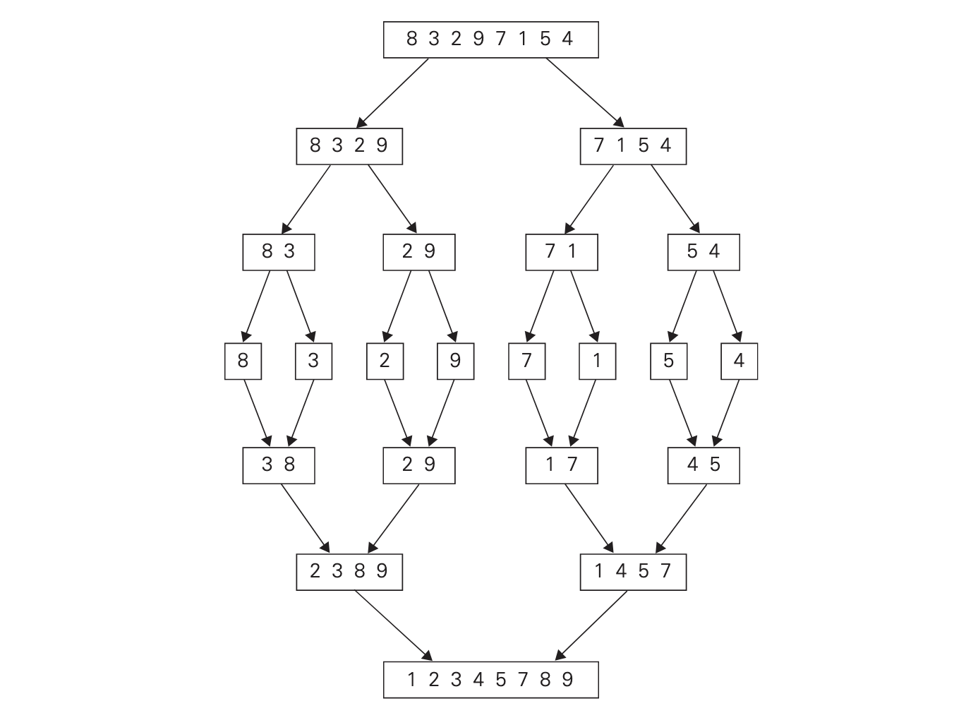
copy B[i ... len(B) - 1] to A[k ... len(B) + len(C) - 1]In the below example of mergesort running on an array [8,3,2,9,7,1,5,4], you can see how it splits the array in halves until it starts to merge them together again in the middle.
Assuming that \(n\) is a power of \(2\), then we can find the recurrence relation for the number of comparisons \(C(n)\).
Take note of the \(C_{\text{merge}}\) in there. It is counting the number of comparisons made in the merge algorithm. In the worst case, neither array becomes empty before the other one, meaning that the algorithm has to compare all items in the arrays and can’t just append the leftover chunk. This means that the number of comparisons the merge step does is \(C_{\text{merge}}(n) = n - 1\), and so our recurrence relation becomes:
Which then, according to the master theorem, means that mergesort has the time complexity of \(\O(n \log{n})\).
Quicksort
Like mergesort, quicksort is another divide-and-conquer algorithm. But, unlike mergesort, quicksort splits the elements in two by their value. Rather than their position as in mergesort. Basically, quicksort selects a pivot point from which it partitions the array into two different arrays: one with all values above the pivot, and one with all values below it. It then recursively repeats the quicksort algorithm on those arrays, meaning that it does all the sorting work when dividing the problem up as opposed to mergesort, where a combination step is required to do the sorting.
function quicksort(A[l ... r]):
    // Input: an array A with its left and right indices defined as l and r
    if l < r:
        // p is the pivot point of the partition
        p <- partition(A[l ... r])
        // runs quicksort on all elements left of the pivot
        quicksort(A[l ... p-1])
        // same for the right side
        quicksort(A[p+1 ... r])
There are two main algorithms that partition the array: Lomuto’s algorithm and Hoare’s algorithm. Here we will discuss Lomuto’s partitioning algorithm because it is pretty easy to understand. Although, it is important to note that Hoare’s algorithm is probably more well known, as they are cited as creating quicksort.
function lomutoPartition(A[l ... r]):
    // input: an array A with its left and right indices defined as l and r
    // output: the newly partitioned array and the position of the pivot point
    p <- A[l]
    s <- l
    for i = l + 1 to r:
        if A[i] < p:
            s <- s + 1
            swap(A[s], A[i])
    // swap the pivot point into its correct position
    swap(A[l], A[s])
return sQuicksort has a worst case time complexity of \(\O(n^2)\). This acutally occurs when the list is already sorted. If quicksort picks a pivot point somewhere near the middle, it will run in \(\Omega(n \log n)\) time.
References
-
[Skiena2020] https://doi.org/10.1007/978-3-030-54256-6_2
-
[Levitin2006] https://dl.acm.org/doi/10.5555/1121708